• Designed and normalized a relational database schema (3NF).
• Implemented many-to-many relationships with junction tables.
• Enforced referential integrity with foreign keys.
• Created complex queries for data aggregation and retrieval.
• Full file(s) available for download on Github!

            
                --Some table Definition Examples

CREATE TABLE CAMPAIGN(
  CID bigint PRIMARY KEY,
  Name varchar(33) NOT NULL,
  campaignBudget real,
  mission text,
  startDate DATE,
  endDate DATE
);

CREATE TABLE DONATES(
  CID bigint,
  DID bigint,
  total real,
  PRIMARY KEY (CID, DID),
  FOREIGN KEY (CID) REFERENCES CAMPAIGN(CID),
  FOREIGN KEY (DID) REFERENCES DONATOR(DID)
);

CREATE TABLE VOLUNTEER (
  VID bigint PRIMARY KEY,
  Name varchar(33) NOT NULL,
  Email varchar(55) NOT NULL,
  tierLevel int,
  Salary real
);

-- Sample insertion into some of the tables

-- campaign
INSERT INTO CAMPAIGN VALUES (100,'green-love',  5000, 'to make trees great again', '2024-03-18', '2024-04-18');
INSERT INTO CAMPAIGN VALUES (101,'generic-protest', 4000, 'we are just protesting to protest', '2024-02-11', '2024-03-02');
INSERT INTO CAMPAIGN VALUES (102, 'idk',  2000,'idk im having trouble coming up with mission statements', '2024-01-02', '2024-02-02');
INSERT INTO CAMPAIGN VALUES (103,'final-countdown',500,'this is the final countdown', '2024-01-02', '2024-02-02');
INSERT INTO CAMPAIGN VALUES (104,'i-just-want-to-slide',2055,'parties in the sky like its 2055', '2055-01-02', '2055-02-02');
-- volunteer
INSERT INTO VOLUNTEER VALUES (927502, 'Clark Davidson', 'clark@gmail.com', 2, 35);
INSERT INTO VOLUNTEER VALUES (927503, 'Dave Hoffman', 'dave@gmail.com',1,NULL);
INSERT INTO VOLUNTEER VALUES (927504, 'Ava Huntington', 'ava@gmail.com', 1,  NULL);
INSERT INTO VOLUNTEER VALUES (927505, 'Clack Clarkson', 'clack@gmail.com',2, NULL);
INSERT INTO VOLUNTEER VALUES (927506, 'Black White', 'black@gmail.com',1,NULL );
INSERT INTO VOLUNTEER VALUES (927507, 'Ivan Naskov', 'ots@gmail.com',2, NULL);
INSERT INTO VOLUNTEER VALUES (927508, 'Debil Naskov', 'Debil@gmail.com',1, NULL);
            
        

• Utilized Psycopg2 for robust PostgreSQL database connections and query execution.
• Designed modular, class-based architecture for maintainability and scalability.
• Implemented dynamic CRUD operations for campaigns, volunteers, and events.
• Created ASCII-based visualizations for financial insights (inflows, outflows, budgets).
• Handled complex SQL queries with Common Table Expressions (CTEs) for data aggregation.
• Incorporated input validation and transaction rollbacks for error handling and data integrity.
• Full file(s) available for download on Github!

            
                # Sample Code: Insert Donations with ON CONFLICT Handling
  
def insertIntoDonatesTable(self):
    tuple_data = (chooseCID, chooseDID, total)
    campaign_data = [tuple_data]
    campsql = """
    INSERT INTO DONATES (CID, DID, total) VALUES (%s, %s, %s)
    ON CONFLICT (CID, DID) DO UPDATE
    SET total = DONATES.total + EXCLUDED.total
    """
    try:
        cursors['cursor6'].executemany(campsql, campaign_data)
        dbconn.commit()
        print("Inserted successfully")
    except psycopg2.Error as e:
        dbconn.rollback()
        print("Error inserting into DONATES table:", e)
            
        

• Implemented a full Scikit-Learn preprocessing pipeline with StandardScaler and OneHotEncoder.
• Utilized DecisionTreeRegressor and RandomForestRegressor for cost prediction.
• Performed hyperparameter tuning with RandomizedSearchCV for model optimization.
• Applied log transformation to normalize skewed distributions.
• Engineered features based on regional, lifestyle, and demographic factors.
• Integrated cross-validation to improve model generalization.
• Full file(s) available for download on Github!

            
                # Scikit-Learn Preprocessing Pipeline for Insurance Cost Prediction

from sklearn.compose import ColumnTransformer
from sklearn.impute import SimpleImputer
from sklearn.preprocessing import StandardScaler, OneHotEncoder
from sklearn.pipeline import make_pipeline
from sklearn.linear_model import LinearRegression

# Define numerical and categorical attributes
num_attribs = ["age", "bmi", "children"]
cat_attribs = ["sex", "smoker", "region"]

# Create transformation pipelines
num_pipeline = make_pipeline(SimpleImputer(strategy="median"), StandardScaler())
cat_pipeline = make_pipeline(SimpleImputer(strategy="most_frequent"), OneHotEncoder(handle_unknown="ignore"))

# Combine pipelines using ColumnTransformer
preprocessing = ColumnTransformer([
    ("num", num_pipeline, num_attribs),
    ("cat", cat_pipeline, cat_attribs)
])

# Create a model pipeline with preprocessing and Linear Regression
model_pipeline = make_pipeline(preprocessing, LinearRegression())

# Train the model
model_pipeline.fit(train_set.drop("charges", axis=1), train_set["charges"])
print("Model trained successfully!")
            
        

• Read and preprocessed data from a CSV file (gpa_year_experience.csv).
• Scaled attributes for better convergence during training.
• Computed and visualized the error at each iteration.
• Predicted new instances and compared results with scikit-learn's SGDRegressor.
• Explored polynomial features to improve predictions.
• Full notebook available for download!

            
                # Linear Regression Implementation Example

import numpy as np
import pandas as pd
import matplotlib.pyplot as plt

# Load the dataset
data = pd.read_csv('gpa_year_experience.csv')

# Feature scaling
data['gpa'] = (data['gpa'] - data['gpa'].mean()) / data['gpa'].std()
data['years_experience'] = (data['years_experience'] - data['years_experience'].mean()) / data['years_experience'].std()

# Initialize weights and bias
weights = np.random.randn(2)
bias = 0
learning_rate = 0.01

# Gradient Descent
for epoch in range(1000):
    predictions = np.dot(data[['gpa', 'years_experience']], weights) + bias
    errors = predictions - data['salary']
    weights -= learning_rate * np.dot(errors, data[['gpa', 'years_experience']]) / len(data)
    bias -= learning_rate * errors.mean()

print("Trained weights:", weights)
print("Trained bias:", bias)

            
        

• Explored the Palmer Penguins dataset with 344 samples across three species.
• Performed data cleaning and preprocessing to handle missing values.
• Visualized relationships between features using scatter plots and histograms.
• Built classification models to predict penguin species based on physical attributes.
• Compared model performance using metrics like accuracy and confusion matrices.
• Full notebook available for download!

            
                # Example: Visualizing the Palmer Penguins Dataset

import pandas as pd
import seaborn as sns
import matplotlib.pyplot as plt

# Load the dataset
penguins = pd.read_csv('penguins.csv')

# Pairplot to visualize relationships between features
sns.pairplot(penguins, hue='species', diag_kind='kde')
plt.show()

# Correlation heatmap
plt.figure(figsize=(10, 6))
sns.heatmap(penguins.corr(), annot=True, cmap='coolwarm')
plt.title('Feature Correlation Heatmap')
plt.show()

            
        

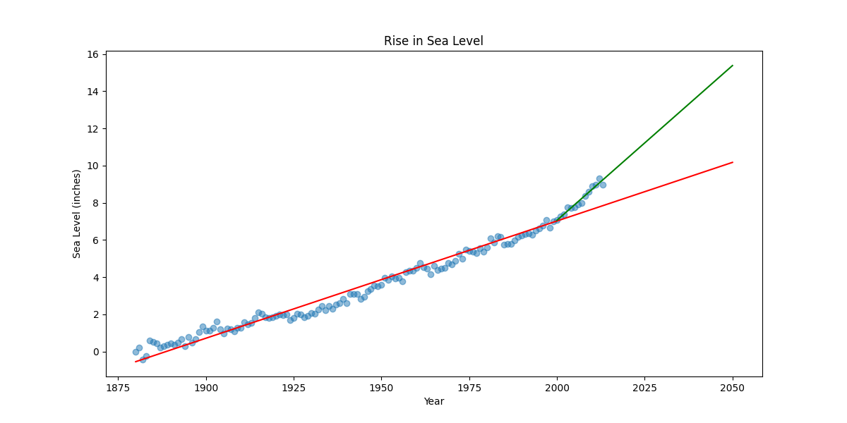
• Loaded and visualized historical sea level data from 1880 to 2013.
• Implemented linear regression to predict sea levels up to 2050.
• Created two lines of best fit: one for all data and one for data since 2000.
• Visualized predictions with scatter plots and regression lines.

Visualization(s)

            
                # Example: Linear Regression for Sea Level Prediction

import pandas as pd
import matplotlib.pyplot as plt
from scipy.stats import linregress

def draw_plot():
    # Read data from file
    df = pd.read_csv("epa-sea-level.csv")
    print(df.head())
    fig, ax = plt.subplots(figsize=(12,6))
    ax.scatter(df["Year"], df["CSIRO Adjusted Sea Level"], label = "Original Data", alpha=0.5)


    # Create first line of best fit and scatter plot
    slope, intercept, r_value, p_value, std_err = linregress(df["Year"],df["CSIRO Adjusted Sea Level"])
    x_vals = pd.Series(range(df['Year'].min(), 2051))
    y_vals = slope *x_vals + intercept

    ax.plot(x_vals, y_vals, 'r', label = f'Best Fit (1880-2050): y = {slope:.4f}x + {intercept:.2f}')
    # Create second line of best fit

    df_recent = df[df['Year'] >= 2000]

    slope_recent, intercept_recent, r_value_recent, p_value_recent, std_err_recent = linregress(df_recent["Year"],df_recent["CSIRO Adjusted Sea Level"])
    x_future = pd.Series(range(2000, 2051))
    y_future = slope_recent * x_future + intercept_recent

    ax.plot(x_future,y_future,'g', label = f'Best Fit (2000-2051): y = {slope_recent:.4f}x + {intercept_recent:.2f}')

    # Add labels and title

    plt.xlabel("Year")
    plt.ylabel("Sea Level (inches)")
    plt.title("Rise in Sea Level")
    
    # Save plot and return data for testing (DO NOT MODIFY)
    plt.savefig('sea_level_plot.png')
    return plt.gca()

            
        

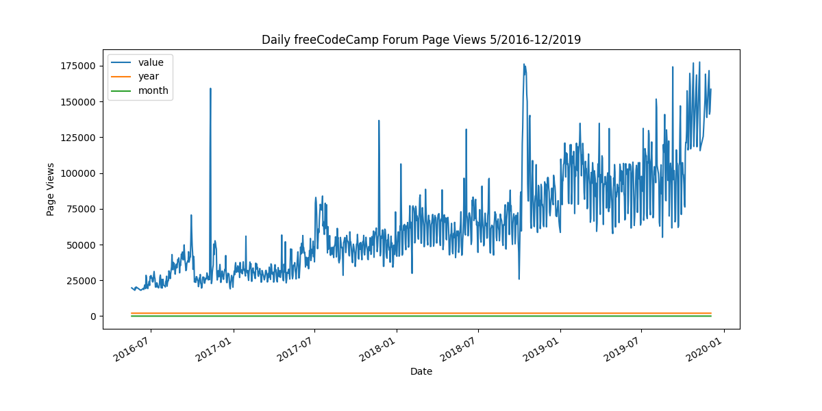
• Cleaned and filtered data to remove outliers.
• Created a line plot to show daily page views over time.
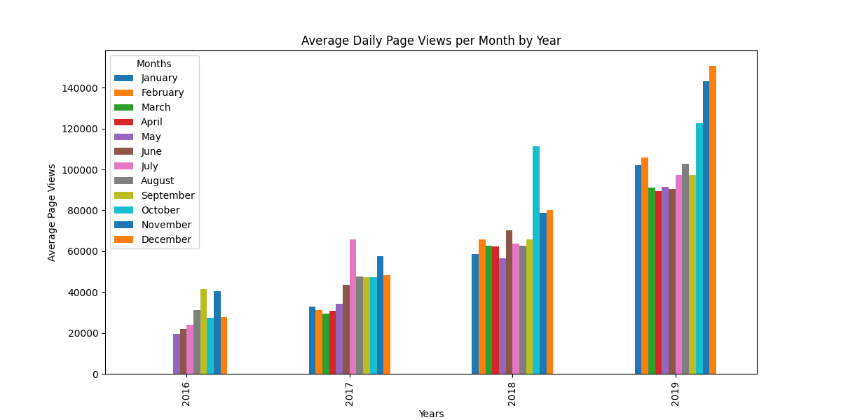
• Generated a bar plot to display monthly averages grouped by year.
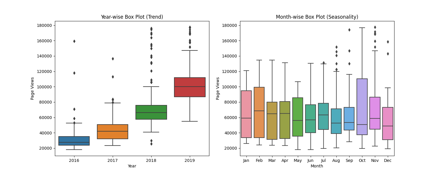
• Designed box plots to visualize yearly and monthly distributions.

Visualization(s)

            
                import matplotlib.pyplot as plt
import pandas as pd
import seaborn as sns
import numpy as np
from pandas.plotting import register_matplotlib_converters
register_matplotlib_converters()

if not hasattr(np, 'float'):
    np.float = float

# Import data (Make sure to parse dates. Consider setting index column to 'date'.)
df = pd.read_csv("fcc-forum-pageviews.csv", parse_dates=["date"], index_col='date')

# Clean data
total_views = df['value'].sum()
df = df[
    (df['value'] < df['value'].quantile(0.975)) &
    (df['value'] > df['value'].quantile(0.025))
]

def draw_line_plot():
    # Draw line plot
    fig = df.plot(figsize=(12, 6), kind='line', title='Daily freeCodeCamp Forum Page Views 5/2016-12/2019', ylabel='Page Views', xlabel='Date').get_figure()
    fig.savefig('line_plot.png')
    return fig

def draw_bar_plot():
    # Copy and modify data for monthly bar plot
    df['year'] = df.index.year
    df['month'] = df.index.month

    # Group by year and month, and calculate the mean daily page views for each month
    monthly_avg = df.groupby(['year', 'month'])['value'].mean().unstack()

    # Plot the bar plot (each month as a separate series)
    ax = monthly_avg.plot.bar(figsize=(12, 6), title='Average Daily Page Views per Month by Year', xlabel='Years', ylabel='Average Page Views')

    # Add legend title and month names directly
    months = ['January', 'February', 'March', 'April', 'May', 'June', 'July', 'August', 'September', 'October', 'November', 'December']
    ax.legend(title='Months', labels=months)

    # Get the figure from the axes object and save the plot
    fig = ax.get_figure()
    fig.savefig('bar_plot.png')
    return fig

def draw_box_plot():
    # Prepare data for box plots
    df_box = df.copy()
    df_box.reset_index(inplace=True)
    df_box['year'] = [d.year for d in df_box.date]
    df_box['month'] = [d.strftime('%b') for d in df_box.date]

    # Draw box plots
    month_order = ['Jan', 'Feb', 'Mar', 'Apr', 'May', 'Jun', 'Jul', 'Aug', 'Sep', 'Oct', 'Nov', 'Dec']
    fig, axes = plt.subplots(1, 2, figsize=(15, 6))
    sns.boxplot(x='year', y='value', data=df_box, ax=axes[0])
    axes[0].set_title('Year-wise Box Plot (Trend)')
    axes[0].set_xlabel('Year')
    axes[0].set_ylabel('Page Views')

    sns.boxplot(x='month', y='value', data=df_box, order=month_order, ax=axes[1])
    axes[1].set_title('Month-wise Box Plot (Seasonality)')
    axes[1].set_xlabel('Month')
    axes[1].set_ylabel('Page Views')

    fig.savefig('box_plot.png')
    return fig

            
        

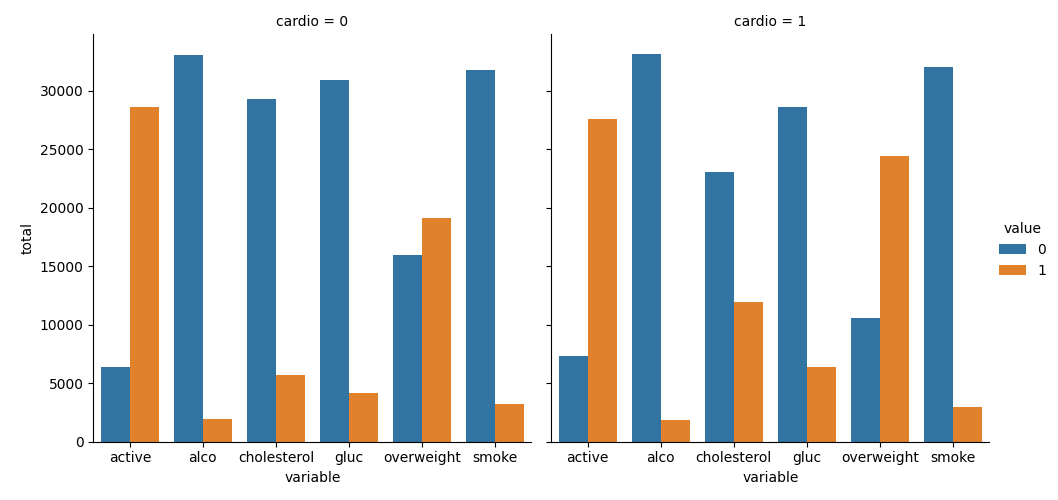
• Calculated BMI to classify individuals as overweight.
• Created categorical plots to compare health metrics by cardiovascular disease status.
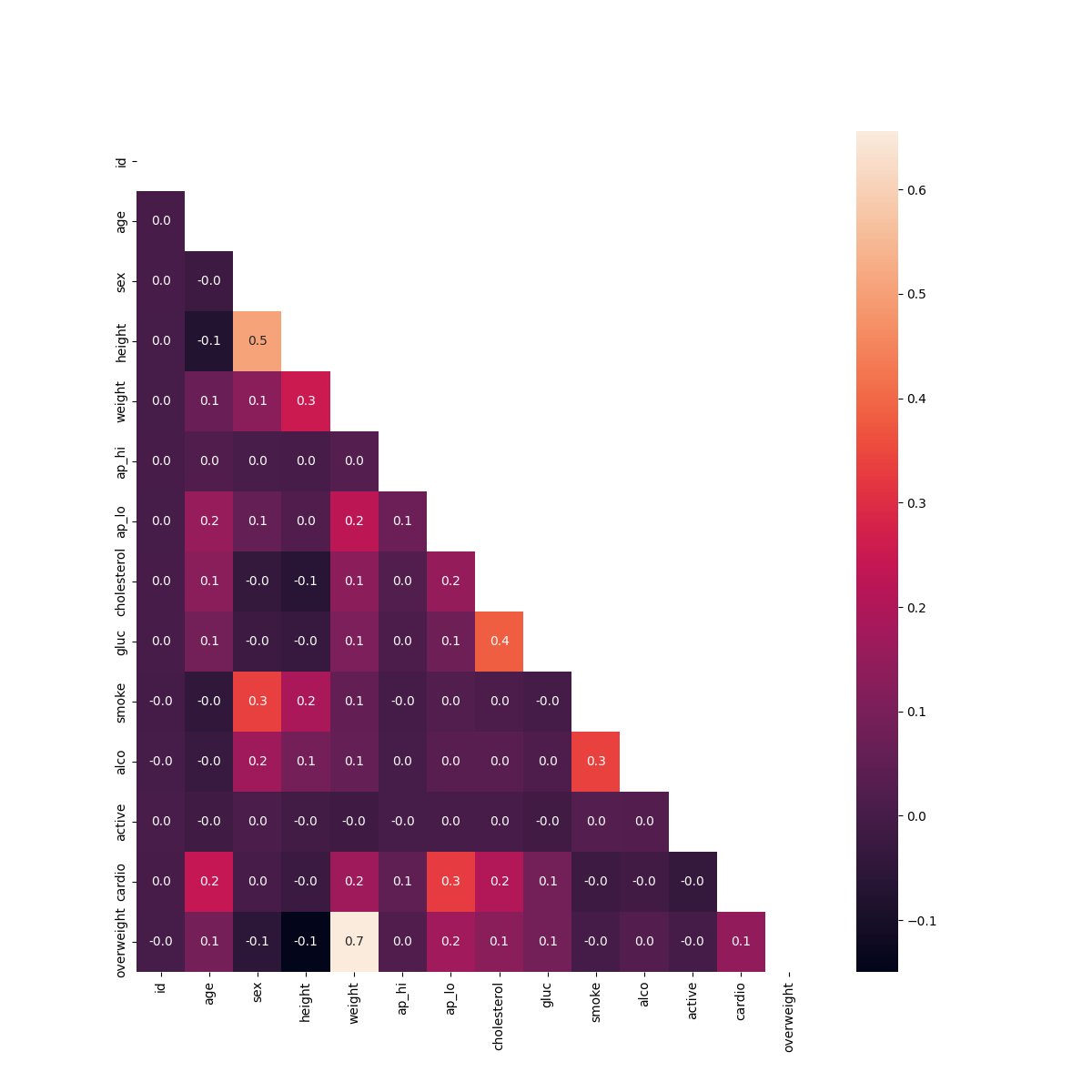
• Generated a heatmap to visualize correlations between health metrics.
• Cleaned data by removing outliers and invalid entries.
• Full script available for download!

Visualization(s)

            
                
import pandas as pd
import seaborn as sns
import matplotlib.pyplot as plt
import numpy as np

df = pd.read_csv("medical_examination.csv")
print(df.head())

df['overweight']=(df['weight'] / (df['height'] / 100) ** 2 > 25).astype(int)
df['cholesterol'] = (df['cholesterol'] > 1).astype(int)
df['gluc'] = (df['gluc'] > 1).astype(int)
print(df.head())

def draw_cat_plot():
    # Create DataFrame for cat plot using `pd.melt` with specified variables
    df_cat = pd.melt(df, id_vars=['cardio'],
                     value_vars=['cholesterol', 'gluc', 'smoke', 'alco', 'active', 'overweight'])

    # Group and reformat the data to split it by 'cardio'
    df_cat = df_cat.groupby(['cardio', 'variable', 'value']).size().reset_index(name='total')
    # Draw the catplot
    fig = sns.catplot(x='variable', y='total', hue='value', col='cardio',
                      data=df_cat, kind='bar').fig
    # Do not modify
    fig.savefig('catplot.png')
    return fig


def draw_heat_map():
    df_heat = df[
        (df['ap_lo'] <= df['ap_hi'])&
        (df['height'] >= df['height'].quantile(0.025))&
        (df['height'] <= df['height'].quantile(0.975))&
        (df['weight'] >= df['weight'].quantile(0.025))&
        (df['weight'] <= df['weight'].quantile(0.975))
    ]

    corr = df_heat.corr()
    mask = np.triu(np.ones_like(corr, dtype=bool))
    fig, ax = plt.subplots(figsize=(12, 12))
    sns.heatmap(corr, mask=mask, annot=True, fmt=".1f", ax=ax)
    fig.savefig('heatmap.png')
    return fig
            
        

• Calculated race representation and average age of men.
• Determined percentages of individuals with advanced education earning >50K.
• Analyzed work hours and income distribution by country.
• Identified the most popular occupation for high earners in India.

            
                # Example: Calculating Demographic Statistics

import pandas as pd

# Load data
df = pd.read_csv("adult.data.csv")

# Calculate statistics
race_count = df['race'].value_counts()
average_age_men = round(df[df['sex'] == 'Male']['age'].mean(), 1)
percentage_bachelors = round((df['education'].value_counts()['Bachelors'] / len(df)) * 100, 1)

print("Race Count:", race_count)
print("Average Age of Men:", average_age_men)
print("Percentage with Bachelors:", percentage_bachelors)

            
        

• Designed and implemented Uniform-Cost Search (UCS) for optimal pathfinding.
• Developed an A* Search algorithm with heuristic evaluation.
• Utilized priority queues for efficient frontier management.
• Implemented graph traversal with state expansion and cost tracking.
• Applied search algorithms to AI-related pathfinding problems.
• Full file(s) available for download on Github!

            
                # A* Search Algorithm Implementation

import heapq

def a_star_search(start, goal, graph, heuristic):
    frontier = []
    heapq.heappush(frontier, (0, start))  # (priority, node)
    came_from = {start: None}
    cost_so_far = {start: 0}

    while frontier:
        _, current = heapq.heappop(frontier)

        if current == goal:
            break

        for neighbor, cost in graph[current]:
            new_cost = cost_so_far[current] + cost
            if neighbor not in cost_so_far or new_cost < cost_so_far[neighbor]:
                cost_so_far[neighbor] = new_cost
                priority = new_cost + heuristic(neighbor, goal)
                heapq.heappush(frontier, (priority, neighbor))
                came_from[neighbor] = current

    return came_from, cost_so_far

# Example Heuristic Function (Manhattan Distance)
def heuristic(node, goal):
    return abs(node[0] - goal[0]) + abs(node[1] - goal[1])

# Example Graph Representation
graph = {
    'A': [('B', 1), ('C', 4)],
    'B': [('A', 1), ('D', 2), ('E', 5)],
    'C': [('A', 4), ('F', 3)],
    'D': [('B', 2)],
    'E': [('B', 5), ('F', 1)],
    'F': [('C', 3), ('E', 1)]
}

came_from, cost_so_far = a_star_search('A', 'F', graph, heuristic)
print("Path cost:", cost_so_far['F'])

            
        

• Implements connection handling for both HTTP (port 80) and HTTPS (port 443).
• Detects HTTP/2 support using ALPN (Application-Layer Protocol Negotiation).
• Parses and extracts cookies from server responses.
• Handles SSL/TLS wrapping for secure connections.
• Includes retry mechanisms and error handling for robust connectivity.
• Full file available for download on Github!

            
                # Snippet: Detecting HTTP/2 Support with ALPN
def upgradeToHttp2(self):
    context = ssl.create_default_context()
    context.set_alpn_protocols(['h2', 'spdy/3', 'http/1.1']) 
    self.s = socket.socket(socket.AF_INET, socket.SOCK_STREAM)
    self.s = context.wrap_socket(self.s, server_hostname=self.domain)
    self.s.connect((self.domain, 443))
    if self.s.selected_alpn_protocol() == "h2":
        return True
    else:
        return False

            
        

• Example 1: Input: nums = [2,7,11,15], target = 9, Output: [0,1]
• Example 2: Input: nums = [3,2,4], target = 6, Output: [1,2]
• Example 3: Input: nums = [3,3], target = 6, Output: [0,1]
• Constraints: 2 <= nums.length <= 10^4, -10^9 <= nums[i], target <= 10^9.
• Full problem description available on <a href='https://leetcode.com/problems/two-sum/' target='_blank' class='text-blue-500 hover:underline'>LeetCode</a>!

            
                # Solution in Python
class Solution:
    def twoSum(self, nums: List[int], target: int) -> List[int]:
        # Create a hash map to store the indices of the numbers
        new_hash = {}
        for x in range(len(nums)):
            value = target - nums[x]
            # Check if the complement exists in the hash map
            if value in new_hash:
                return [new_hash[value], x]
            # Store the current number and its index in the hash map
            new_hash[nums[x]] = x
        return None

            
        

• Example 1: Input: strs = ["flower","flow","flight"], Output: "fl"
• Example 2: Input: strs = ["dog","racecar","car"], Output: "" (No common prefix).
• Constraints: 1 <= strs.length <= 200, 0 <= strs[i].length <= 200.
• Full problem description available on <a href='https://leetcode.com/problems/longest-common-prefix/' target='_blank' class='text-blue-500 hover:underline'>LeetCode</a>!

            
                # Solution in Python
class Solution:
    def longestCommonPrefix(self, strs: List[str]) -> str:
        # Find the shortest string length
        min_length = float('inf')
        i = 0
        for x in strs:
            if len(x) < min_length:
                min_length = len(x)
        # Compare characters across strings
        while i < min_length:
            for s in strs:
                if s[i] != strs[0][i]:
                    return s[:i]
            i += 1
        return strs[0][:i]

            
        

• Example 1: Input: nums = [1,3,5,6], target = 5, Output: 2
• Example 2: Input: nums = [1,3,5,6], target = 2, Output: 1
• Example 3: Input: nums = [1,3,5,6], target = 7, Output: 4
• Constraints: 1 <= nums.length <= 10^4, -10^4 <= nums[i] <= 10^4.
• nums contains distinct values sorted in ascending order.
• Full problem description available on <a href='https://leetcode.com/problems/search-insert-position/' target='_blank' class='text-blue-500 hover:underline'>LeetCode</a>!

            
                # Solution in Python
class Solution:
    def searchInsert(self, nums: List[int], target: int) -> int:
        low = 0
        high = len(nums) - 1
        while low <= high:
            mid = low + (high - low) // 2
            if nums[mid] == target:
                return mid
            elif nums[mid] < target:
                low = mid + 1
            else:
                high = mid - 1
        if target < nums[mid]:
            return mid
        else:
            return mid + 1

            
        

• Example 1: Input: numbers = [2,7,11,15], target = 9, Output: [1,2]
• Example 2: Input: numbers = [2,3,4], target = 6, Output: [1,3]
• Example 3: Input: numbers = [-1,0], target = -1, Output: [1,2]
• Constraints: 2 <= numbers.length <= 3 * 10^4, -1000 <= numbers[i] <= 1000.
• numbers is sorted in non-decreasing order.
• Your solution must use only constant extra space.
• Full problem description available on <a href='https://leetcode.com/problems/two-sum-ii-input-array-is-sorted/' target='_blank' class='text-blue-500 hover:underline'>LeetCode</a>!

            
                # Solution in Python
class Solution:
    def twoSum(self, numbers: List[int], target: int) -> List[int]:
        ptr1 = 0
        ptr2 = len(numbers) - 1
        while ptr1 < ptr2:
            if target < numbers[ptr2] + numbers[ptr1]:
                ptr2 -= 1
            if numbers[ptr2] + numbers[ptr1] < target:
                ptr1 += 1
            if numbers[ptr2] + numbers[ptr1] == target:
                if ptr1 <= ptr2:
                    return [ptr1+1, ptr2+1]
                else:
                    return [ptr2+1, ptr1+1]
        return []

            
        

• Example 1: Input: nums = [1,1,1,0,0,0,1,1,1,1,0], k = 2, Output: 6
• Example 2: Input: nums = [0,0,1,1,0,0,1,1,1,0,1,1,0,0,0,1,1,1,1], k = 3, Output: 10
• Constraints: 1 <= nums.length <= 10^5, nums[i] is either 0 or 1, 0 <= k <= nums.length.
• Full problem description available on <a href='https://leetcode.com/problems/max-consecutive-ones-iii/' target='_blank' class='text-blue-500 hover:underline'>LeetCode</a>!

            
                # Solution in Python
class Solution:
    def longestOnes(self, nums: List[int], k: int) -> int:
        max_window = 0
        num_zeros = 0
        l = 0
        
        for r in range(len(nums)):
            if nums[r] == 0:
                num_zeros += 1
            
            while num_zeros > k:
                if nums[l] == 0:
                    num_zeros -= 1
                l += 1
            
            temp_window = r - l + 1
            if temp_window > max_window:
                max_window = temp_window
        
        return max_window

            
        

• Implemented pixel rendering for a 16x16 grid using MIPS assembly.
• Utilized nested loops for row-major traversal of a byte array.
• Converted binary values (0/1) to pixel colors (black/white).
• Managed stack and registers for function calls in a low-level environment.
• Full file available for download on Github!

            
                # draw_16x16:
# $a0: start address of 16x16 byte array
# Renders array to bitmap display (0 = black, 1 = white)
draw_16x16:
    addi $sp, $sp, -16
    sw $ra, 0($sp)
    sw $s0, 4($sp)
    sw $s1, 8($sp)
    sw $s2, 12($sp)
    
    add $s0, $zero, $a0    # Source array
    add $s1, $zero, $zero  # Row counter
draw_row:
    add $s2, $zero, $zero  # Column counter
draw_col:
    add $a0, $zero, $s0
    add $a1, $zero, $s1
    add $a2, $zero, $s2
    jal get_16x16          # Get byte value (0 or 1)
    
    add $a0, $zero, $s1    # Row
    add $a1, $zero, $s2    # Col
    sub $a2, $zero, $v0    # 0 -> 0x00000000, 1 -> 0xffffffff
    jal set_pixel          # Draw pixel
    
    addi $s2, $s2, 1
    blt $s2, 16, draw_col
    addi $s1, $s1, 1
    blt $s1, 16, draw_row
    
    lw $ra, 0($sp)
    lw $s0, 4($sp)
    lw $s1, 8($sp)
    lw $s2, 12($sp)
    addi $sp, $sp, 16
    jr $ra